Abstract

Agricultural production in Brazil has increasingly relied on groundwater extraction, raising concerns about the sustainability of underground reservoirs. This paper compares the diffusion of the two most common types of wells used to extract groundwater for agriculture in the state of São Paulo, Brazil: conventional (low depth) and tubular (high depth). We use longitudinal municipal-level information and spatial panel models to analyze the two main drivers of groundwater extractions: climate variability (aridity) and environmental conservation (conservation agriculture and native forest conservation). Our results highlight how increasing aridification in the dry season (winter) has reduced the diffusion of conventional wells and increased the diffusion of less sustainable tubular wells. We also highlight that soil conservation and native forest preservation practices reduce the need for deep underground water extraction.

Keywords: Soil conservation, forest conservation, econometrics, peer relationship, São Paulo.

JEL Classification: Q25, Q50, C01.

Resumen

En Brasil, la producción agrícola depende cada vez más de la extracción de agua subterránea. Ello genera preocupaciones sobre la sostenibilidad de las reservas subterráneas. Así pues, este artículo compara la difusión de los dos tipos de pozo más comunes para extraer agua del subsuelo para la agricultura, en el estado de São Paulo: convencional (baja profundidad) y tubular (alta profundidad). Se usaron datos longitudinales de nivel municipal y modelos de panel espacial, a fin de analizar los dos principales estimuladores de la extracción de agua subterránea: la variabilidad climática (aridez) y la conservación ambiental (agricultura de conservación y conservación de flora nativas). Los resultados destacan que la creciente aridez en la estación seca (invierno) ha reducido la difusión de pozos convencionales y ha aumentado la difusión de pozos tubulares menos sostenibles. A su vez, las prácticas de conservación del suelo y los bosques nativos reducen la necesidad de extracción de aguas subterráneas profundas.

Palabras clave: conservación de suelos, conservación de bosques, econometría, relación entre pares, São Paulo.

Clasificación JEL: Q25, Q50, C01.

Introduction

Groundwater resources1 play a fundamental role in the hydrological cycle. Studies indicate that about 98% of the world’s freshwater are in underground reservoirs (Margat and Gun, 2013), and about 33% of the water used globally comes from underground reservoirs (Famiglietti, 2014). Brazil presents some of the most important sources of groundwater in the world. The National Aeronautics and Space Administration (NASA) indicates that three of the 37 principal aquifers worldwide are located in Brazil: Amazon Basin, Maranhão Basin, and Guarani Aquifer System (NASA/JPL-Caltech, 2020). The country extracts nearly 17.6 million cubic meters of groundwater per year, one-quarter intended for the agricultural sector consumption (Hirata et al., 2019).

In recent decades, reserves depletion has become a global-scale problem as groundwater growing usage has reduced reserves worldwide (Villar and Villar, 2016; Wada et al., 2010). Groundwater contamination by chemical compounds, mostly from agricultural activities, is another grave concern (Margat and Gun, 2013). Part of the underground water reservoirs corresponds to geological formations that are non-renewable (FAO, 2003), whose inappropriate use can imply permanent depletion of the water resources. The groundwater depletion involves the excessive appropriation and uses resulted from individual and collective decisions. As a freely accessible resource, groundwater appropriation relates to the tragedy of the commons, i.e., the intensive exploitation of a shared resource by one of few users acting according to their self-interest (Hardin, 1968; Ostrom, 2012).

Two key recent changes in agriculture help explaining the sustainability or depletion of groundwater reservoirs. The first is climate change, which may impose additional threats to groundwater reservoirs. Global dependence on groundwater for water consumption and food security tends to increase as a response to increasing temperature and more frequent and intense extreme droughts events (Hirata and Conicelli, 2012; Treidel et al., 2012). In turn, little is yet known about how underground reservoirs respond to climatic variations and how climate change has the potential to affect aquifers’ hydrogeological processes (Green et al., 2011; Margat and Gun, 2013). Haldorsen et al. (2011) suggest that air and river temperature variability can influence the aquifers’ temperatures and oxygen concentrations, impairing water quality.

The second change is environmental conservation, which is a way to mitigate the impacts of climate change on groundwater reservoirs (Kløve et al., 2014). For example, conservationist agricultural practices would allow better water infiltration in the soil, favoring the groundwater replenishment and the aquifers’ water quality (Kassam et al., 2019a). Native forests may also favor hydrological processes, such as evapotranspiration, soil moisture, and recharge of surface and groundwater systems, stabilizing seasonal courses and reducing soil erosion and rainwater runoff (Warziniack et al., 2017).

This paper analyzes how climate variability and environmental preservation relate to the diffusion of underground wells among agricultural producers in the state of São Paulo (SP), Brazil. We compare the diffusion of the two most common types of wells in SP: conventional (low depth dub/bored wells) and tubular (high depth driven or drilled wells). We use longitudinal data with municipal-level information for the years 2006 and 2017. Our empirical strategy uses spatial panel models to test different hypotheses about the diffusion of more and less sustainable groundwater extraction practices among neighbor farmers. This strategy allows us to consider the existence of environmental spillovers, i.e., that the impacts and benefits of climate variability and environmental conservation practices go beyond the municipal borders.

The evidence found suggests that climate variability is related to the greater diffusion of high-depth wells. However, greater use of conservational and native forest preservation practices would generate greater resilience to climate variations, and would therefore be associated with lower diffusion of tubular wells. The importance of the neighborhood’s effect on local decisions on groundwater extraction was also demonstrated through the existence of spillover effects on the diffusion of underground wells.

SP is a singular case to analyze climate variability and environmental conservation impacts on groundwater consumption in agriculture. Its modern agriculture positioned this highly dynamic state as the second most significant value of agricultural production in Brazil (IBGE, 2020). Throughout its historical land use, native forests have gradually converted to agricultural areas and pasture, compromising the supply of surface water for agriculture (Gori Maia et al., 2018). In this context, the SP aquifers represent an essential provider of steady freshwater supply for agriculture and human consumption, especially the Guarani aquifer, the second largest in the world (SMA, 2012). Nevertheless, its tropical and humid climate combined with an abundant supply of surface water may not avoid challenges posed by extreme climate events such as the severe water crisis SP faced in 2014 (Côrtes et al., 2015; Villar and Villar, 2016).

In addition to this introduction, the paper is divided into five sections. The second section presents a review of the literature. The third section presents the data source, variables, and the empirical strategy based on spatial panel data models. The fourth section presents the results, which are discussed in detail in the fifth section. The last section presents the final considerations and their implications in terms of the sustainability of the water resource, as well as the limitations of the study.

I. Theoretical background

The economic literature about groundwater use has focused on analyzing the water market development, addressing price determinants, market structure, negotiation strategies, and governance mechanisms (Khair et al., 2019). Special attention has given to variables related to the farmers’ socioeconomic characteristics, the type of economic activity and water supply (Li and Zhao, 2018), the agricultural systems’ characteristics, the production technologies (Singh and Park, 2018), land ownership, association, and extension services (Mekonnen et al., 2016). Few studies have analyzed how climate change or conservation practices may affect groundwater use in agriculture.

Most studies on the relationship between climate variability and groundwater focus on the supply side. Kløve et al. (2014) indicated that the impacts of climatic variability depend on underground reservoirs’ size and recharge flows. Recharge flows would also depend on the distribution and amount of precipitation, losses due to evapotranspiration, the type of soil cover, and the water table level (Scibek et al., 2007). Furthermore, rising temperature increases evaporative demand over surface, which reduces the amount of water to replenish the aquifers (Wu et al., 2020). Ludwing and Moench (2009) argued that substantial climate variations would affect recharge and, hence, the reservoirs’ volume and depth. These variations would also increase the water extraction from low recharge reservoirs, significantly lowering groundwater levels (Treidel et al., 2012).

The characteristics of underground water reservoirs may also be crucial for the sustainability of water use in agriculture. Small and shallow unconfined systems2 are more sensitive and respond quickly to climate change, as they are more likely to have renewable groundwater. In turn, confined reservoirs3 present a slower response due to a relevant proportion of non-renewable groundwater (Lee et al., 2006). According to Wada et al. (2012), non-renewable groundwater resources may be the most vulnerable to the effects of increased extraction to meet current consumption needs and future water demand in a context of climatic variability. Hornbeck and Keskin (2014) point out that, in the short term, greater access to groundwater makes agriculture less sensitive to droughts by increasing the intensity of irrigation. In the long term, farmers shift to more water-intensive crops, which increases sensitivity to climate variability (due to depletion of underground reserves). Therefore, for the authors, the net impact of groundwater on drought sensitivity is theoretically ambiguous.

Studies have more recently focused on how agricultural management practices may affect the sustainability of groundwater used for irrigation (Wada et al., 2010). Conservation agriculture seems to offer an alternative to optimize the use of natural resources through integrated soil management, water resources, and ecosystem services (Kassam et al., 2019a). According to Zhang and Schilling (2006), soil conservation practices would alter water’s temporal and spatial use, allowing greater efficiency by reducing evapotranspiration and runoff losses. Therefore, they could also impact the underground reservoirs’ recharge flows. Hornbeck and Keskin (2014) argue that, in water-scarce regions, the use of agricultural practices that minimize water consumption would be related to mitigating agricultural sensitivity to climate variability.

Dakhlalla et al. (2016) simulated the groundwater reservoirs’ recharge with various types of soil conservation practices. The authors found that conservation practices affected the amount of recharge in aquifers by decreasing the extraction flow and favoring water infiltration into the soil. Ni et al. (2020) simulated the adoption of conservation agriculture practices and found a positive association between conservation practices and the water table level recovery: conservation practices would allow more efficient use of water resources and reduce underground reservoirs’ depletion. However, Klocke et al. (1999) found no significant differences between conservation and conventional practices outcomes in groundwater use in corn and soy plantations in Nebraska.

The preservation of native forests is a critical component of conservation agriculture. Native forests provide a wide range of ecosystem services (ES), such as carbon sequestration, runoffs, water quality, and flood control (De Groot et al., 2002). According to Neary et al. (2009), forests reduce rainwater runoff, preventing soil water erosion. Furthermore, the dense network of native vegetation roots acts as a filter reducing pollutant levels that could contaminate the water tables. Warziniack et al. (Warziniack et al., 2017) argue that the native forest is the best soil cover for regulating seasonal flows and ensuring high groundwater quality under any hydrological and ecological circumstances.

Krishnaswamy et al. (2013) indicated that the underground reservoir load is positively influenced by the natural forest areas regardless of the water balance4. Paul (2006) analyzed aquifers in the west of Jilin province in China and observed higher recharges in native vegetation areas, while pasture or bare areas would associate with more water table deterioration. Zhang and Hiscock (2010) found that the decrease in groundwater volume depends on the vegetation type, the soil characteristics, and the climatic conditions.

Despite the aforementioned studies, the relationships between climate variability, environmental preservation, and the use of underground water resources still a line of research poorly addressed in the literature. One main contribution of this article is to understand these associations in a developing country, where, to the best of our knowledge, there is not yet empirical work of this nature.

II. Material and methods

A. Dependent variables

We use longitudinal data with information from all 645 municipalities in SP in two years, 2006 and 2017. The primary source of information is the Brazilian Agricultural Census, conducted by the Brazilian Institute of Geography and Statistics (IBGE) in 2006 and 2017. The census interviewed 227 622 farms in SP in 2006 and 188 643 in 20175. Since census farm-level information was not publicly available, we aggregated this information into the 645 municipalities in SP.

We compute two dependent variables from the census: the proportion of farms with conventional wells; the proportion of farms with tubular or artesian wells6. Conventional wells have a maximum depth of 40 meters (IBGE, 2009). Conventional wells are holes in the ground able to reach the beginning of the water table, which is the first water reserve closest to the surface. Conventional wells are more susceptible to contamination by chemical and biological agents (Costa and Rozza, 2015) and subject to climatic variability7. Tubular wells are constructed by driving pipes into the ground to capture water from the deep groundwater reserves. They can use gushers or pumping systems; their depth varies from 50 to 2000 meters, so they would not need filters to retain impurities (Gaber, 2005). Between 2006 and 2017, the average municipal percentage of farms in SP using common wells decreased from 34.6% to 24.4%, while those with tubular wells increased from 21.9% to 41.1%.

Conventional wells are spatially concentrated in the SP eastern region, near the state’s most populous and developed area (Figure 1). According to DAEE and UNESP (DAEE and UNESP, 2013), this region presents a rich supply of surface water resources (such as rivers, springs, and lagoons). The aquifers are mainly located above crystalline basement rocks, whose geological properties make it challenging to access groundwater. The tubular wells are spatially concentrated in the western region, which has enormous groundwater potential due to the Paraná Basin’s sedimentary rocks, whose characteristics contribute to higher volume storage, ease of access, and transport (Akie and Ezaki, 2012). We used spatial lags of the dependent variables and errors (to be explained below) to control the spatial concentration in the distribution of wells.

Conventional Wells 2006

Conventional Wells 2017

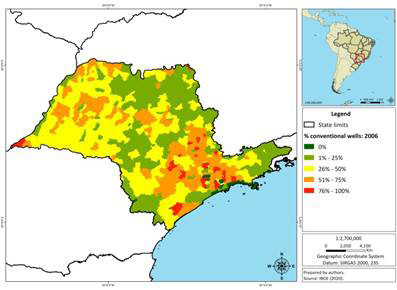
Tubular Wells 2006

Tubular Wells 2017

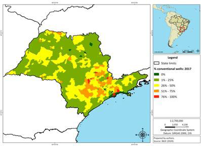
Source: Data from CNA 2006/2017.

B. Independent variables7

This study focuses on two main drivers of groundwater diffusion: climatic variability and environment conservation. The indicator of climatic variability comes from data provided by the Instituto Nacional de Meteorologia (INMET, 2017). Based on Genius et al. (Genius et al., 2014), we computed a proxy for aridity given by the ratio between the municipal average annual temperature and the total average annual precipitation. This aridity index allows us to capture the combined effect of temperature and precipitation, for example, how droughts may accentuate the effects of high temperatures. We standardized the aridity index to control historical differences between municipalities (Dell et al., 2014). The standardized aridity index is given by the difference between the average aridity in the reference period and the historical average since 1970, divided by the standard deviation since 1970. The reference period covers the prior ten years of each census, i.e., 1996-2005 for the Census 2006 and 2007-2016 for the Census 2017. The historical period excludes the reference period, i.e., 1970-1995 for the Census 2006 and 1970-2006 for the Census 2017. Such periodicity allows us to capture long-term responses to climatic variations (Sampson and Perry, 2019).

The predominant climate in the state of SP is tropical. Therefore, it was necessary to calculate the standardized aridity index for the coldest and driest season (winter, April to September) and the hottest and wet season (summer, between October and March). This allows for a better capture of the relationships between climate variability and the diffusion of groundwater wells (Morales et al., 2022). Table 1 shows that the aridity was exceptionally high in the dry season between 1996-2005 (0.462) and particularly low in the wet season of the same reference period (-0.266).

Aridity Index – Wet Season 2006

Aridity Index – Wet Season 2017

Aridity Index – Dry Season 2006

Aridity Index – Dry Season 2017

Source: Data from CNA 2006/2017 and INMET 2020.

Figure 2 shows the spatial distribution of the average aridity index in the reference period for each year of the Agricultural Census (2006 and 2017). It can be seen that in almost all municipalities in the state of SP, the wet season became more arid from 2006 to 2017. However, the Western region shows a greater number of municipalities with increased aridity. This result is mainly explained by the decrease in the level of precipitation experienced by the state of SP (Figure 3). According to Morales et al. (2022), the wet season (summer) is one of crop growth and, therefore, agricultural producers in a scenario of falling precipitation would require greater water resources, since adequate water conditions are necessary for the proper development of seedlings. This would be related to the decrease in conventional wells and the increase in tubular wells, as a measure of adaptation to climate variability (Figure 1). On the contrary, the dry season became less arid from 2006 to 2017, yet the highest levels of aridity continued to be recorded in the western region of the state of SP (Figure 2). This dynamic can be explained mainly by the increase in precipitation along the state territory, at a time that is naturally of little rain (Figure 3). The temperature was relatively stable in the dry season, and was characterized by registering higher levels in the Western region relative to the Eastern region, which may explain the higher aridity index in the West, and its spatial concentration of greater-depth wells (Figure 4).

Precipitation – Wet Season 2006

Precipitation – Wet Season 2017

Precipitation – Dry Season 2006

Precipitation – Dry Season 2017

Source: Data from CNA 2006/2017 and INMET 2020.

Temperature – Wet Season 2006

Temperature – Wet Season 2017

Temperature – Dry Season 2006

Temperature – Dry Season 2017

Source: Data from CNA 2006/2017 and INMET 2020.

We defined two indicators of environmental conservation: conservation practices in agriculture and native forest cover. The first indicator, conservation agriculture, is based on Maia et al. (Gori Maia et al., 2018). We applied principal component analysis (PCA) to the share of the five most-used soil conservation practices in SP between 2006 and 2017 (IBGE, 2009, 2018b): no-till farming on straw (3.0% and 7.4%, respectively, in 2006 and 2017), minimum tillage (9.7% and 15%), contour farming (44% and 38%), fallow (4% and 15%), and crop rotation (9% and 23%). We selected the first common factor of the PCA, representing about 40% of the total variability of the five variables above. Table 4 in the Appendix shows the factorial loads and the scoring coefficients associated with the first common factor. Except for contour farming, all variables showed positive correlations with the selected factor, with correlation coefficients ranging from 0.51 (no-till in straw) to 0.87 (crop rotation). Our indicator of conservation practices is a binary variable assuming for municipalities with a factor score above the 75th percentile and 0 otherwise8. The proportion of municipalities above the 75th percentile in 2006 and 2017 is 8.4% and 41%, respectively (Table 1).

Our second indicator of environmental comes from maps of land cover provided by MapBiomas (MapBiomas, 2020). First, we computed the average proportion of the municipal area covered with native forest for 1996-2005 (reference for 2006) and 2007-2016 (reference for 2017). Second, we generated a binary variable assuming 1 for municipalities with an average of native forest above the 75th percentile and 0 otherwise9. The proportion of municipalities with the largest share of the native forest increased from 23.4% in 2006 to 26.6% in 2017 (Table 1).

Our control variables are based on the prior studies, and therefore incorporate the recommendations of the specialized literature on the subject (Khair et al., 2019; Li and Zhao, 2018; Mekonnen et al., 2016; Singh and Park, 2018): type of agricultural activity (proportion of farms with temporary crop, permanent crop, and livestock); proxy for surface water supply (log of the municipal water bodies area); water storage (proportion of farms with cisterns); farmer’s characteristics (proportion of farmers by educational level, age group, sex, and management type); social and environmental characteristics (proportion of family farms, organic farms, and members of cooperatives, class entities or farmers’ association); energy access (proportion of farms with access to electricity); technical assistance (proportion of farms receiving technical guidance); land tenure (proportion of farms that are owned by the own farmer, rented, transferred or occupied); soil correction and fertilization (proportion of farms that used soil pH correction, and fertilization); employment and production (log of the number of employees and the value of the previous year production10 of farms with temporary crops, permanent crops, and livestock); credit (proportion of farms receiving credit for investment, costing, and maintenance); mechanization (proportion of farms with tractors or other machines); area (proportion of farms by groups of area).

The main changes between 2006 and 2017 are related to (Table 1): educational attainment (the share of farmers with at least secondary education increased from 32% to 44%); aging (the share of aged 65 and more increased from 22% to 30%); membership in farmers association (the share of members of cooperatives increased from 17% to 26%); fertilizers (the share of farms using fertilizers increased from 51% to 60%); area (the share of farms with an area between 50 and 500 hectares increased from 8.4% to 20.1%).

C. Empirical Strategy

Our benchmark model assumes that the diffusion of underground water for agriculture is a function of environmental and socioeconomic characteristics (equation 1):

\[ P_{jit} = \alpha_t + \mathbf{Z}_{it}' \boldsymbol{\delta}_j + \mathbf{X}_{it}' \boldsymbol{\beta}_j + c_i + \varepsilon_{jit} \tag{1}\]

Where \( P_{jit} \) is the proportion of farms at municipality \( i \) and year \( t \) with the \( j \)-th type of underground well (\( j = 1 \) for conventional wells and \( j = 2 \) for artesian or tubular wells); \( \mathbf{Z} \) is a vector of environmental variables (aridity, conservation agriculture, and forest preservation); \( \mathbf{X} \) is a vector of control variables. Our primary interest is the vector \( \boldsymbol{\delta} \), which contains the coefficients defining the net impacts of environmental variables on the diffusion of each type of underground water. The vector \( \boldsymbol{\beta} \) contains the coefficients for the control variables. The factor \( c_i \) represents the unobserved municipal heterogeneity that is constant over time (e.g., access to groundwater reservoir), and is controlled for via fixed effects (within transformation). The time-varying intercept \( \alpha_t \) represents changes between census years that are common across municipalities (e.g., macroeconomic cycles affecting agricultural production), and is controlled using a binary variable that takes the value 1 in 2017. Finally, \( \varepsilon_{jit} \) is the idiosyncratic random error.

One main limitation of equation (1) is the assumption that the diffusion of underground water in one municipality is independent of the diffusion of underground water or environmental conservation in other municipalities. However, Figure 1 suggests that the diffusion of underground water is spatially concentrated in SP. Prior studies have also suggested the existence of peer effects or spillovers in groundwater extraction. i.e., the farm’s decision to use groundwater may be influenced by other farms’ decisions (Sampson and Perry, 2018). We tested the existence of spatial dependence in the diffusion of groundwater extraction using different specifications of spatial models (Anselin, 2001). A more traditional specification of spatial model is the SAR (Spatial Autoregressive) model: \[ P_{jit} = \alpha_t + \rho_j \mathbf{w}_i' P_{jt} + \mathbf{z}_{it}' \boldsymbol{\delta}_j + \mathbf{x}_{it}' \boldsymbol{\beta}_j + c_{i} + \varepsilon_{jit} \tag{2} \] Where the spatial neighborhood matrix \( \mathbf{w}_i \) contains positive values for municipalities with common borders, excluding vertex (Rook’s contiguity criterion), and zero otherwise. These positive values are equal to the inverse of the distance: \(\frac{1}{d_{ij}^b}\) where \( d_{ij} \) is the distance (in km) between municipalities \( i \) and \( j \). The vector \( P_{jt} \) contains the proportion of farms in each municipality using the \( j \)-th type of underground well in period \( t \). The SAR model assumes that the proportion of underground wells in municipality \( i \), \( P_{jit} \), is influenced by the average proportion in neighboring municipalities \( \mathbf{w}_i' P_{jt} \) (Anselin, 2003). The spatial autocorrelation coefficient \( \rho_j \) represents the spatial dependence between the diffusion of the \( j \)-th underground well in municipality \( i \) and the diffusion in its neighbors (LeSage, 2008). This coefficient is restricted \(|\rho| < 1 \) to avoid an explosive behavior of the spatial association (LeSage, 2008).

We also tested the sensitiveness of our estimates using other spatial model specifications. The SAC (Spatial Autocorrelation) model assumes that the diffusion of underground wells in municipality \( i \) is influenced by diffusion in the neighborhood and unobserved factors in the neighborhood (Fingleton, 2008). The SDM (Spatial Durbin Model) assumes that the diffusion of underground wells in municipality \( i \) is influenced by diffusion in the neighborhood and average environmental characteristics in the neighborhood (LeSage and Pace, 2009). The GSM (General Spatial Model) assumes that the diffusion of underground wells in municipality \( i \) is simultaneously influenced by diffusion in the neighborhood, unobserved factors in the neighborhood, and average environmental characteristics in the neighborhood.

We estimate equation (1) using the generalized least squares (GLS) method, assuming municipal heterogeneity. We estimate equation (2) and other spatial models using the quasi-maximum likelihood (QML) method, which obtains consistent and asymptotically more efficient estimators in the presence of spatial lags (Lee, 2004). The likelihood log function in the QML estimation of spatial models controls the potential endogeneity of the spatial dependence term (Bell and Bockstael, 2000). It means that this strategy would consider Manski’s reflection problem (Manski, 1993), given by the simultaneity of interaction between observations. In this sense, the spatial estimation by QML would provide efficient and consistent estimates (Tsusaka et al., 2015).

III. Results

A. Spatial clusters and main estimates

The diffusion of agricultural groundwater use in SP shows strong patterns of spatial dependence (Figure 5). The LISA clusters (Local Indicator of Spatial Association) (Anselin, 2010) identify the groups of municipalities with similar or opposite proportions of farms with conventional and tubular wells each year. The high-high cluster aggregates municipalities with a high proportion (above average) of one type of well and surrounded by municipalities with a high proportion of the same type of wells. The high-high clusters for common wells are concentrated in the SP eastern region and, for tubular wells, in the western region. The low-low cluster aggregates municipalities with low proportions (below average) surrounded by municipalities with low proportions. The low-low clusters for conventional wells are spatially spread out, while those for tubular wells are concentrated in the SP eastern. The high-low and the low-high aggregate a few spatial outliers, i.e., municipalities with proportions that are the opposite of those in the neighborhood.

Conventional Wells 2006

Conventional Wells 2017

Tubular Wells 2006

Tubular Wells 2017

Source: Data from CNA 2006/2017, PAM 2005/2016, INMET and MapBiomas 2020.

Table 2 shows the estimates of equation (1) and spatial models for conventional and tubular wells. We present all the results obtained, in order to check the sensitiveness of econometric estimates, to the different functional specifications and empirical strategies proposed. According to the BIC information criterion, the best model for both conventional and tubular wells is the SAR. The likelihood ratio confirms that the spatial dependence increases the goodness of fit for both models (conventional and tubular wells). In fact, the literature regarding groundwater extraction (Koch and Nax, 2017; Sampson and Perry, 2019, 2018) suggests that there are primarily endogenous associations with the neighborhood, which are statistically significant in decision-making on the extraction of water resources. The SAR model reflects this structure of endogenous dependence and the spatial interrelationship between the municipalities. We will henceforth focus our analyses to the SAR model11.

The models fitted better for tubular wells, with coefficients of determination (R2-within) ranging between 68% and 70% (between 42% and 43% for conventional wells). The spatial lags are significant in all spatial models, with greater magnitude (higher spatial correlation) in the case of tubular wells. In other words, our estimates show that the spatial spillover effect is more intense for tubular wells than for common wells.

Our results indicate that aridity and agricultural conservation practices significantly explain the diffusion of underground wells. The estimates for the aridity index are significant in the models without spatial lags (GLS) and in the SAR and SAC models. These estimates suggest that each increase of one standard deviation in aridity index during the dry season implies that: (i) the municipal proportion of farms with conventional wells decreases between 0.068 and 0.094 percentage points (p.p.); (ii) the proportion of farms with tubular wells increases between 0.056 and 0.092 p.p. In turn, the increase of one standard deviation in the aridity index during the wet season (summer) would be positively associated with the diffusion of conventional wells (variation between 0.069 and 0.117 p.p. %) and negatively associated with the diffusion of tubular wells (variation between -0.056 and -0.135 p.p.).

The estimates for conservation agriculture are significant in models GLS, SAR, SDM, and GSM. These estimates indicate that the greater the diffusion of conservationist agricultural practices, the lower the diffusion of conventional wells (negative estimates between 0.026 and 0.029). In turn, the impacts of conservation agriculture on the diffusion of tubular wells are insignificant. We also did not find evidence that the share of native forest in the municipality may significantly affect the diffusion of conventional and tubular wells.

The estimates for the spatial lags indicate that the diffusion of common and tubular wells depends on the diffusion in neighboring municipalities (endogenous peer effect) and unobservable factors in the neighborhood (correlated peer effect). The estimates for the lags of environmental conservation in the neighborhood are insignificant in most models.

B. Heterogeneous effects and decomposition of spatial effects

To analyze potential heterogeneous effects in the extraction of groundwater resources, we now interact the aridity index with conservation practices and native forest conservation (Table 3). The idea is to check to what extent environmental conservation may mitigate the influence of climatic variability on the diffusion of underground water use.

The interaction between the aridity index in the dry season and the conservation agriculture is statistically significant on the diffusion of tubular wells. Specifically, the relationship between dry season´s aridity and the diffusion of tubular wells is 0.051 p.p. lower on those municipalities with the largest use of agricultural conservation practices.

We also decomposed the SAR models' estimates into direct, indirect, and total spatial components (Table 4). This strategy considers that environmental changes can potentially affect the diffusion of wells at both the municipality and the neighborhood (LeSage and Pace, 2009), this would show the importance of neighborhood relations in the diffusion pattern of groundwater extraction. The direct component represents the effect of environmental changes at the municipal level. The indirect component represents the local effect of environmental changes at neighboring municipalities. We are particularly interested in analyzing the indirect component, which represent the spillover effects of environmental changes in the neighborhood.

The indirect component represents about 27% of the estimated coefficient between aridity variability and the diffusion of conventional wells. This means that part of this relationship is explained by the climate variability of neighboring municipalities. During the dry season, the diffusion of conventional wells at the municipality level decreases by 0.031 percentage points for each one standard deviation increase in aridity in neighboring municipalities. During the wet season, it increases by 0.017 percentage points. Moreover, the diffusion of conventional wells decreases by 0.011 percentage points in neighborhoods with a high proportion of conservationist agricultural practices. This indirect effect corresponds to nearly 30% of the estimated coefficient for this relationship.

IV. Discussion

This study shows that environmental changes may be significantly associated with the diffusion of underground wells. We analyzed the case of SP, the state with the second-largest agricultural production in Brazil and a rich groundwater supply. The use of tubular wells for irrigation in SP increased by 19 p.p. between 2006 and 2017, while the use of conventional wells reduced by 10 p.p. Our results show that the diffusion of less sustainable tubular wells was associated with increases in the aridity during the driest season (winter). Low precipitation and high temperature may affect the recharge flows and underground reservoirs’ volume and depth (Ludwing and Moench, 2009). Small, shallow systems are more quickly affected by increasing aridity, which restricts the use of conventional wells for irrigation (Lee et al., 2006) and pressures deeper reserves with tubular wells to meet current and future demands (Treidel et al., 2012). The results shown may have been driven by the water crisis presented by the state of SP in 2014 (which affected dozens of cities in the countryside, in addition to the main drinking water production systems), which was characterized as an extreme climatic event12 with a drastic drop in the region’s average rainfall, but also as a water supply crisis caused by the exceptional drought of that year. In the wet season (summer) of 2013 – 2014, droughts and high temperatures that surpassed several records occurred in several regions of the state of SP, which led to an increase in the aridity index (Ambrizzi and Coelho, 2018).

Aridity changes during the wet season (summer) show opposite relationships those of the dry season (winter): increases in aridity during the wet season were positively associated with the diffusion of conventional wells and negatively associated with the diffusion of tubular wells. This result may be related to the seasonal variations of the water table (Jasechko et al., 2014). The recharging of the Guaraní Aquifer System’s reservoirs, which is the primary source of groundwater in SP, takes place in the rainy months, between October and March (Lucas et al., 2015). Decreases in precipitation during the rainy months may compromise the recharge of deeper reservoirs and, thus, the diffusion of tubular wells (Healy and Cook, 2002).

While climatic changes in SP were associated with increased diffusion of tubular wells, environmental conservation showed to be a key factor in attenuating the increasing demand for shallow and deep groundwater. The diffusion of conservation practices in agriculture, such as no-till, minimum tillage, fallow, and crop rotation, increased by 33 points between 2006 and 2017. Increases in conservation practices were associated with lower diffusion of conventional wells. In addition, the evidence found also suggests that the municipalities of SP, most of which use this type of agricultural practice, seem to be more resilient to the effects of climate variability in the dry season, and therefore would be able to mitigate (reduce) the increase in tubular wells as an adaptive measure to climate change. These two results could be related, according to Kassam et al. (2019b), to the benefits derived from conservational agriculture by allowing for better optimization of natural resources through integrated soil management. For example, conservational practices would favor better use of water resources by decreasing the rates of loss due to evapotranspiration and runoff, which would modify the pattern of temporal and spatial water usage, thus avoiding the depletion of groundwater due to a lower adoption of lesser- and greater-depth wells (Ni et al., 2020).

The diffusion of tubular wells as a response to increasing aridity during the wet season was lower in municipalities with the largest share of native forests: the estimate for interaction between aridity during the wet season and native forest preservation was negative and significant. Native forest may increase climatic resilience by increasing direct rain catchment, favoring the production and maintenance of surface water flows (Brauman et al., 2012). This natural forest eco-hydrological function plays a critical role, influencing the shape, water quantity, and quality transported to river basins (Neary et al., 2009). Moreover, the native vegetation provides a suitable microclimate for the springs maintenance, streams, or smaller bodies of water, reducing the incidence of sunlight and the water flow variation due to climatic events such as droughts or floods (Warziniack et al., 2017).

The estimates for the spatial lags highlight the importance of the peer effects on the underground water resources diffusion. Peer effects represent the knowledge and experience transmission among nearby localities, highlighting the spatial interdependence in the diffusion of agricultural practices (Richards, 2018). Koch and Nax (2017) and Sampson and Perry (Sampson and Perry, 2018) found similar results regarding aquifers’ exploration. These results show that informal mechanisms of information transmission, based on neighborhood relations, are relevant factors that must be considered to understand the adoption of underground wells (Batagelj et al., 2014). The endogenous peer effect (spatial lag of the dependent variable) was stronger for tubular wells than conventional ones, suggesting that the spatial concentration is more frequent for tubular wells. Finally, the spatial coefficients decomposition shows the relevance of the neighborhood in local decisions on groundwater extraction. Nearly one-third of the total relationships analyzed with the diffusion of wells at the municipal level were manifested through the indirect effect of spatial spillovers, i.e., through environmental changes that took in the neighborhood.

V. Final remarks

Analyses of the factors determining underground well adoption are fundamental to support public policy formulation to protect and sustain water resources in the long term. These policies may be essential to reduce the increasing demand for tubular wells in SP, partially responding to climatic changes in the state. In this regard, this paper point out that climate variability in the dry season (winter in SP) is related to changes in the pattern of groundwater extraction. Small, near-surface reservoirs would be rapidly affected, decreasing the use of conventional wells. This would increase the pressure to exploit greater-depth water resources (tubular wells) to meet consumption demands, which could compromise the water table level. In turn, climate variability in the wet season (summer in SP) would potentially affect the seasonal refill regime of the deeper aquifers, which would alter the subsoil water removal scheme by increasing the spread of common wells and decreasing that of tubulars.

Another relevant result of our analyses is that greater use of conservational agricultural practices is associated with a decrease in conventional wells, and a high proportion of native forest conservation areas, which may generate greater resilience to climate variations, reduces the diffusion of tubular wells as an adaptive measure. The evidence found also highlights the importance of the influence of the neighborhood on groundwater extraction decisions. Tubular wells have a higher pattern of spatial concentration, which may intensify the exploration of deep aquifers and affect the water regime of neighboring locations. This would generate a behavior of conditional reciprocity as a response to the overexploitation of neighbors (peer effect or spatial spillover), which would accelerate the extraction of non-renewable water resources, compromising the sustainability of the water table.

It is important to mention that the results found in this research do not necessarily reflect a causal relationship but rather establish associations between climatic and environmental conditions and the diffusion of wells for groundwater extraction. These results allowed us to draw some conclusions about the sustainable use of water resources during a water crisis in SP. However, we can not generalize these results because some municipalities may have had a peculiar trend during this period. For example, municipalities that have been more affected by climate variations during the analysis period might already present a specific trend in the diffusion of adaptation strategies. Another limitation is that our analyses are limited to the period of availability of data from the Brazilian Agricultural Census (2006 and 2017). Further studies might advance the analysis using, for example, a broader period and reinforce the causal relationships between the variables.

Acknowledgments

This research was supported by the Coordenação de Aperfeiçoamento de Pessoal de Nível Superior (CAPES, grant number 88887.115961/2016-01)

This research was the result of the doctoral thesis “Peer effects in water resources consumption: the São Paulo state experience”, by Daniel Morales Martínez at the State University of Campinas–Braz il.

We would like to thank Reviewers for taking the necessary time and effort to review the manuscript. We sincerely appreciate all your valuable comments and suggestions, which helped us in improving the quality of the manuscript.

Footnotes:

References

1. Akie, M., Ezaki, S. (2012). As Águas Subterrâneas do Estado de São Paulo, Cadernos de Educação Ambiental – Secretaria do Meio Ambiente.
2. Ambrizzi, T., & Coelho, C. (2018). A crise hídrica e a seca de 2014 e 2015 em São Paulo: contribuições do clima e das atividades humanas. In A crise hídrica na região metropolitana de São Paulo em 2013–2015: Origens, impactos e soluções, Livro Branco da Água (p. 175). São Paulo.
3. Anselin, L. (2010). Local indicators of spatial association–LISA. Geographical Analysis, 27, 93–115. https://doi.org/10.1111/j.1538-4632.1995.tb00338
4. Anselin, L. (2003). Spatial externalities, spatial multipliers, and spatial econometrics. International Regional Science Review, 26(2), 153–166. https://doi.org/10.1177/0160017602250972
5. Anselin, L. (2001). Spatial econometrics. In B. H. Baltagi (Ed.), A companion to theoretical econometrics (pp. 310–330). Blackwell Publishing Ltd.
6. Batagelj, V., Doreian, P., Ferligoj, A., & Kejžar, N. (2014). Understanding large temporal networks and spatial networks: Exploration, pattern searching, visualization and network evolution. Wiley. https://doi.org/10.1002/9781118915370
7. Bell, K. P., & Bockstael, N. E. (2000). Applying the generalized-moments estimation approach to spatial problems involving microlevel data. Review of Economics and Statistics, 82(1), 72–82. https://doi.org/10.1162/003465300558641
8. Brauman, K. A., Freyberg, D. L., & Daily, G. C. (2012). Land cover effects on groundwater recharge in the tropics: ecohydrologic mechanisms. Ecohydrology, 5(4), 435–444. https://doi.org/10.1002/eco.236
9. Côrtes, P. L., Torrente, M., Pinto Alves Pinto, A., Ruiz, M. S., Dias, A. J. G., & Rodrigues, R. (2015). Crise de abastecimento de água em São Paulo e falta de planejamento estratégico. Estudos Avançados, 29(84), 7–26. https://doi.org/10.1590/S0103-40142015000200002
10. Costa, A. F., & Rozza, G. (2015). Recursos hídricos subterrâneos: análise de poços de Rodeio (SC). Revista Eletrônica do Alto Vale do Itajaí, 3(4), 78–81. https://doi.org/10.5965/2316419003042014078
11. DAEE & UNESP. (2013). Águas subterrâneas no Estado de São Paulo: Diretrizes de utilização e proteção. Secretaria de Saneamento e Recursos Hídricos, São Paulo.
12. Dakhlalla, A. O., Parajuli, P. B., Ouyang, Y., & Schmitz, D. W. (2016). Evaluating the impacts of crop rotations on groundwater storage and recharge in an agricultural watershed. Agricultural Water Management, 163, 332–343. https://doi.org/10.1016/j.agwat.2015.10.001
13. De Girolamo, A. M., Bouraoui, F., Buffagni, A., Pappagallo, G., & Lo Porto, A. (2017). Hydrology under climate change in a temporary river system: Potential impact on water balance and flow regime. River Research and Applications, 33(8), 1219–1232. https://doi.org/10.1002/rra.3165
14. De Groot, R. S., Wilson, M. A., & Boumans, M. J. (2002). A typology for the classification, description and valuation of ecosystem functions, goods and services. Ecological Economics, 41(3), 393–408. https://doi.org/10.1016/S0921-8009(02)00089-7
15. Dell, M., Jones, B. F., & Olken, B. A. (2014). What do we learn from the weather? The new climate-economy literature. Journal of Economic Literature, 52(3), 740–798. https://doi.org/10.1257/jel.52.3.740
16. EPA. (2020). Groundwater.
17. Famiglietti, J. S. (2014). The global groundwater crisis. Nature Climate Change, 4, 945–948. https://doi.org/10.1038/nclimate2425
18. FAO. (2003). Review of World Water Resources by Country (1st ed.). Food and Agriculture Organization of the United Nations, Rome.
19. Ferreira, J. L., Ruffoni, J., & Carvalho, A. M. (2018). Dinâmica da difusão de inovações no contexto brasileiro. Revista Brasileira de Inovação, 17(1), 175–200. https://doi.org/10.20396/rbi.v16i4.8650852
20. Fingleton, B. (2008). A generalized method of moments estimator for a spatial panel model with an endogenous spatial lag and spatial moving average errors. Spatial Economic Analysis, 3(1), 27–44. https://doi.org/10.1080/17421770701774922
21. Gaber, M. (2005). Michigan Flowing Well Handbook. Michigan Department of Environmental Quality, Water Bureau.
22. Genius, M., Koundouri, P., Nauges, C., & Tzouvelekas, V. (2014). Information transmission in irrigation technology adoption and diffusion: Social learning, extension services, and spatial effects. American Journal of Agricultural Economics, 96(1), 328–344. https://doi.org/10.1093/ajae/aat054
23. Gori Maia, A., Miyamoto, B. C. B., & Garcia, J. R. (2018). Climate change and agriculture: Do environmental preservation and ecosystem services matter? Ecological Economics, 152, 27–39. https://doi.org/10.1016/j.ecolecon.2018.05.013
24. Green, T. R., Taniguchi, M., Kooi, H., Gurdak, J. J., Allen, D. M., Hiscock, K. M., Treidel, H., & Aureli, A. (2011). Beneath the surface of global change: Impacts of climate change on groundwater. Journal of Hydrology. https://doi.org/10.1016/j.jhydrol.2011.05.002
25. Haldorsen, S., Heim, M., & Van Der Ploeg, M. (2011). Impacts of climate change on groundwater in permafrost areas: Case study from Svalbard, Norway. In Climate change effects on groundwater resources: A global synthesis of findings and recommendations (pp. 323–338). CRC Press. https://doi.org/10.1201/b11611
26. Hardin, G. (1968). The tragedy of the commons. The population problem has no technical solution; it requires a fundamental extension in morality. Science, 162(3859), 1243–1248. https://doi.org/10.1126/science.162.3859.1243
27. Healy, R. W., & Cook, P. G. (2002). Using groundwater levels to estimate recharge. Hydrogeology Journal, 10(1), 91–109. https://doi.org/10.1007/s10040-001-0178-0
28. Hirata, R., & Conicelli, B. P. (2012). As águas subterrâneas e sua importância ambiental e econômica para o Brasil. Anais da Academia Brasileira de Ciências, 84(2), 297–312. https://doi.org/10.11606/9788563124074
29. Hirata, R., Suhogusoff, A. V., Marcellini, S. S., Villar, P. C., & Marcellini, L. (2019). Estudos de Águas Subterrâneas. São Paulo.
30. Hornbeck, R., & Keskin, P. (2014). The historically evolving impact of the Ogallala Aquifer: Agricultural adaptation to groundwater and drought. American Economic Journal: Applied Economics, 6(1), 190–219. https://doi.org/10.1257/app.6.1.190
31. IBGE. (2020). Sistema IBGE de Recuperação Automática – SIDRA. IBGE – Instituto Brasileiro de Geografia e Estatística.
32. IBGE. (2018a). Censo Agro 2017: Resultados preliminares mostram queda de 2,0% no número de estabelecimentos e alta de 5% na área total. Agência IBGE – Notícias. https://agenciadenoticias.ibge.gov.br/agencia-sala-de-imprensa/2013-agencia-de-noticias/releases/21905
33. IBGE. (2018b). Produção Agrícola Municipal 2018. Instituto Brasileiro de Geografia e Estatística.
34. IBGE. (2009). Censo Agropecuário 2006 – Brasil, grandes regiões e unidades da federação. Instituto Brasileiro de Geografia e Estatística, Rio de Janeiro.
35. INMET. (2017). Portal do INMET – Instituto Nacional de Meteorologia.
36. Jasechko, S., Birks, S. J., Gleeson, T., Wada, Y., Fawcett, P. J., Sharp, Z. D., McDonnell, J. J., & Welker, J. M. (2014). The pronounced seasonality of global groundwater recharge. Water Resources Research, 50, 8845–8867. https://doi.org/10.1002/2014WR015809
37. Kassam, A., Friedrich, T., & Derpsch, R. (2019a). Global spread of conservation agriculture. International Journal of Environmental Studies, 76(1), 29–51. https://doi.org/10.1080/00207233.2018.1494927
38. Kassam, A., Friedrich, T., & Derpsch, R. (2019b). Global spread of conservation agriculture. International Journal of Environmental Studies, 76(1), 29–51. https://doi.org/10.1080/00207233.2018.1494927
39. Khair, S. M., Mushtaq, S., Reardon-Smith, K., & Ostini, J. (2019). Diverse drivers of unsustainable groundwater extraction behaviour operate in an unregulated water-scarce region. Journal of Environmental Management, 236, 340–350. https://doi.org/10.1016/j.jenvman.2018.12.077
40. Klocke, N. L., Watts, D. G., Schneekloth, J. P., Davison, D. R., Todd, R. W., & Parkhurst, A. M. (1999). Nitrate leaching in irrigated corn and soybean in a semi-arid climate. Transactions of the ASAE, 42(6), 1621–1630. https://doi.org/10.13031/2013.13328
41. Kløve, B., Ala-Aho, P., Bertrand, G., Gurdak, J. J., Kupfersberger, H., Kværner, J., Muotka, T., Mykrä, H., Preda, E., Rossi, P., Uvo, C. B., Velasco, E., & Pulido-Velazquez, M. (2014). Climate change impacts on groundwater and dependent ecosystems. Journal of Hydrology, 518, 250–266. https://doi.org/10.1016/j.jhydrol.2013.06.037
42. Koch, C., & Nax, H. (2017). Groundwater usage: Game theory and empirics.
43. Krishnaswamy, J., Bonell, M., Venkatesh, B., Purandara, B. K., Rakesh, K. N., Lele, S., Kiran, M. C., Reddy, V., & Badiger, S. (2013). The groundwater recharge response and hydrologic services of tropical humid forest ecosystems to use and reforestation: Support for the “infiltration–evapotranspiration trade-off hypothesis.” Journal of Hydrology, 498, 191–209. https://doi.org/10.1016/j.jhydrol.2013.06.034
44. Lee, L., Lawrence, D., & Price, M. (2006). Analysis of water-level response to rainfall and implications for recharge pathways in the Chalk aquifer, SE England. Journal of Hydrology, 330, 604–620. https://doi.org/10.1016/j.jhydrol.2006.04.025
45. Lee, L.-F. (2004). Asymptotic distributions of quasi-maximum likelihood estimators for spatial autoregressive models. Econometrica, 72(6), 1899–1925. https://doi.org/10.1111/j.1468-0262.2004.00558.x
46. LeSage, J. P. (2008). An introduction to spatial econometrics. Revue d’économie industrielle, 123, 19–44.
47. LeSage, J. P., & Pace, R. K. (2009). Introduction to spatial econometrics. CRC Press.
48. Li, H., & Zhao, J. (2018). Rebound effects of new irrigation technologies: The role of water rights. American Journal of Agricultural Economics, 100(3), 786–808. https://doi.org/10.1093/ajae/aay001
49. Lucas, M., Oliveira, P. T. S., Melo, D. C. D., & Wendland, E. (2015). Évaluation de données de télédétection pour estimer la recharge d’une zone d’affleurement du Système Aquifère de Guarani (Amérique du Sud). Hydrogeology Journal, 23, 961–969. https://doi.org/10.1007/s10040-015-1246-1
50. Ludwing, F., & Moench, M. (2009). The impacts of climate change on water. In F. Ludwing, P. Kabat, H. Van Schaik, & M. Van der Valk (Eds.), Climate Change Adaptation in the Water Sector (pp. 35–50). Earthscan Publishing.
51. Manski, C. F. (1993). Identification of endogenous social effects: The reflection problem. The Review of Economic Studies, 60(3), 531–542. https://doi.org/10.2307/2298123
52. MapBiomas. (2020). Coleção 5 da Série Anual de Mapas de Cobertura e Uso de Solo do Brasil. https://mapbiomas.org (accessed 9.1.20).
53. Margat, J., & Van der Gun, J. (2013). Groundwater around the World: A Geographic Synopsis (1st ed.). CRC Press.
54. Mekonnen, D., Siddiqi, A., & Ringler, C. (2016). Drivers of groundwater use and technical efficiency of groundwater, canal water, and conjunctive use in Pakistan’s Indus Basin Irrigation System. International Journal of Water Resources Development, 32(3), 459–476. https://doi.org/10.1080/07900627.2015.1133402
55. Morales, D., Gori-Maia, A. G., & Garcia, J. (2022). Spatial diffusion of efficient irrigation systems: A study of São Paulo, Brazil. Australian Journal of Agricultural and Resource Economics, 66(3), 690–712. https://doi.org/10.1111/1467-8489.12483
56. NASA/JPL-Caltech. (2020). Map of Groundwater Storage Trends for Earth’s 37 Largest Aquifers. Jet Propulsion Laboratory, California Institute of Technology.
57. Neary, D. G., Ice, G. G., & Jackson, C. R. (2009). Linkages between forest soils and water quality and quantity. Forest Ecology and Management, 258(10), 2269–2281. https://doi.org/10.1016/j.foreco.2009.05.027
58. Ni, X., Parajuli, P. B., & Ouyang, Y. (2020). Assessing agriculture conservation practice impacts on groundwater levels at watershed scale. Water Resources Management, 34, 1553–1566. https://doi.org/10.1007/s11269-020-02526-3
59. Ostrom, E. (2012). The challenge of crafting rules to change open access resources into managed resources. SSRN Electronic Journal, Workshop in Political Theory and Policy Analysis, Bloomington, p. 29. https://doi.org/10.2139/ssrn.1936109
60. Paul, M. J. (2006). Impact of land-use patterns on distributed groundwater recharge and discharge – A case study of western Jilin, China. Chinese Geographical Science, 16(3), 229–235. https://doi.org/10.1007/s11769-006-0229-5
61. Richards, P. (2018). It’s not just where you farm; it’s whether your neighbor does too. How agglomeration economies are shaping new agricultural landscapes. Journal of Economic Geography, 18(1), 87–110. https://doi.org/10.1093/jeg/lbx009
62. Sampson, G. S., & Perry, E. D. (2019). Peer effects in the diffusion of water-saving agricultural technologies. Agricultural Economics, 50(5), 693–706. https://doi.org/10.1111/agec.12518
63. Sampson, G. S., & Perry, E. D. (2018). The role of peer effects in natural resource appropriation – The case of groundwater. American Journal of Agricultural Economics, 101(1), 154–171. https://doi.org/10.1093/ajae/aay090
64. Scibek, J., Allen, D. M., Cannon, A. J., & Whitfield, P. H. (2007). Groundwater–surface water interaction under scenarios of climate change using a high-resolution transient groundwater model. Journal of Hydrology, 333(2–4), 165–181. https://doi.org/10.1016/j.jhydrol.2006.08.005
65. Singh, S., & Park, J. (2018). Drivers of change in groundwater resources: A case study of the Indian Punjab. Food Security, 10, 965–979. https://doi.org/10.1007/s12571-018-0823-2
66. SMA. (2012). As águas subterrâneas do estado de São Paulo. Cadernos de Educação Ambiental, Governo do Estado de São Paulo – Secretaria do Meio Ambiente.
67. Treidel, H., Martin-Boordes, J., & Gurdak, J. (2012). Climate Change Effects on Groundwater Resources: A Global Synthesis of Findings and Recommendations. Taylor & Francis Publishing.
68. Tsusaka, T. W., Kajisa, K., Pede, V. O., & Aoyagi, K. (2015). Neighborhood effects and social behavior: The case of irrigated and rainfed farmers in Bohol, the Philippines. Journal of Economic Behavior & Organization, 118, 227–246. https://doi.org/10.1016/j.jebo.2015.04.022
69. Villar, P. C., & Villar, P. C. (2016). Groundwater and the right to water in a context of crisis. Ambiente & Sociedade, 19, 85–102. https://doi.org/10.1590/1809-4422asoc150126r1v1912016
70. Wada, Y., Van Beek, L. P. H., & Bierkens, M. F. P. (2012). Nonsustainable groundwater sustaining irrigation: A global assessment. Water Resources Research, 48. https://doi.org/10.1029/2011WR010562
71. Wada, Y., Van Beek, L. P. H., Van Kempen, C. M., Reckman, J. W. T. M., Vasak, S., & Bierkens, M. F. P. (2010). Global depletion of groundwater resources. Geophysical Research Letters, 37. https://doi.org/10.1029/2010GL044571
72. Warziniack, T., Sham, C. H., Morgan, R., & Feferholtz, Y. (2017). Effect of forest cover on water treatment costs. Water Economics and Policy, 3(4), 1750006. https://doi.org/10.1142/S2382624X17500060
73. Wu, W.-Y., Lo, M.-H., Wada, Y., Famiglietti, J. S., Reager, J. T., Yeh, P. J.-F., Ducharne, A., & Yang, Z.-L. (2020). Divergent effects of climate change on future groundwater availability in key mid-latitude aquifers. Nature Communications, 11, 3710. https://doi.org/10.1038/s41467-020-17581-y
74. Zhang, H., & Hiscock, K. M. (2010). Modelling the impact of forest cover on groundwater resources: A case study of the Sherwood Sandstone aquifer in the East Midlands, UK. Journal of Hydrology, 392, 136–149. https://doi.org/10.1016/j.jhydrol.2010.08.002
75. Zhang, Y. K., & Schilling, K. E. (2006). Effects of land cover on water table, soil moisture, evapotranspiration, and groundwater recharge: A field observation and analysis. Journal of Hydrology, 319, 328–338. https://doi.org/10.1016/j.jhydrol.2005.06.044

Appendix