Introduction
Potatoes are one of the most widely grown crops in the world (faostat, 2019), but yield losses might occur due to diseases and pests. Among these, late blight disease stands out. Caused by the oomycete Phytophthora infestans (P. infestans), late blight is a destructive disease of potato (Solanum tuberosum and S. tuberosum group phureja) in the tropics and the most important pathogen of this species and other Solanaceous plants worldwide (Kanetis et al., 2010). In Colombia, the first official reports of the disease were published by Chardon (1928) in the late 1920s. The use of fungicides is the main strategy implemented to control the emergence and spread of epidemics, but its extensive use greatly damages the environment, increases production costs, and in some cases causes crop abandonment in emerging countries (Harrison & Lowe, 1989). For this reason, the development of resistant cultivars as an alternative strategy to control this disease is important to potato growers and researchers (Erwin & Ribeiro, 1996; Fry, 2008). Additionally, researchers seek to understand climate variables that control epidemic dynamics to guide the application of fungicides with forecast models. These models are used to indirectly estimate late blight severity by determining the number of fungicide applications needed during the growing season (Hijmans et al., 2000). This approach requires the integration of information regarding pathogen biology, the effect of the environment on pathogen fitness, and host resistance/susceptibility.
P. infestans presents both asexual and sexual sporulation. In Colombia, the sexual phase has not been reported and, although Vargas et al. (2009) detected mating type A2 in addition to the already reported type A1, no sexual recombination has been conclusively demonstrated thus far (Cárdenas et al., 2011). The asexual phase begins in the tuber or in foliage lesions and is followed by the production of sporangia and direct germination in certain conditions, whereas in other conditions zoospores are produced by indirect germination (Judelson, 1997). Weather conditions directly and indirectly influence the asexual phase of P. infestans. Temperature has been shown to modulate germination (Crosier, 1934; Harrison & Lowe, 1989). Humidity also has a major effect on disease development in potato plant foliage because it affects two key stages in the life cycle of P. infestans: i) the production of sporangia, and ii) germination leading to infection (Harrison & Lowe, 1989). The prolonged survival of sporangia and their formation also requires high relative humidity (Harrison, 1992; Harrison & Lowe, 1989). In another study, a correlation was found between humidity and the number of diseased leaflets of tomato and potato plants under field conditions (Lima et al., 2009). Rainfalls increase the availability of free water in the atmosphere, affecting humidity and water on foliage surface. Without free water on the leaf surface, zoospores cannot be released from zoosporangia since they are unable to swim and, therefore, infection cannot occur (Crosier, 1934). Under heavy rain conditions, spore dispersal is favored because zoospores inside droplets can be transported short distances within the plot (MacKenzie et al., 1983).
The isolated study of these variables can provide helpful insights on possible disease behavior in the field. However, interactions between these environmental conditions may uniquely influence local conditions in the field, affecting thus pathogen behavior. To the best of our knowledge, there are no models of the field conditions of P. infestans sporulation that collectively consider the following variables: rainfall, temperature, solar radiation, relative humidity, and dew point. Additionally, with a continued measurement of these variables, it is possible to calculate their historical trends, describe long-term behavior, and detect weather anomalies—meteorological parameters that deviate from the historical mean (ideam, 2006)1. Indeed, weather variables not always comply with the expected patterns and in some cases climate data show anomalies that should be considered in disease models. For example, due to the weakness of trade winds, the Humboldt Current is faint, which generates an accumulation of warm water in the western Pacific and an upwelling zone on the South American coast. Because the Humboldt Current is diminishing, the movement of warm surface water from east to west is weakened, resulting in the phenomena known as “El Niño.” The opposite phenomenon, known as “La Niña,” is characterized by lower-than-average temperatures in the surface waters of the eastern Pacific Ocean because the Humboldt Current has strengthened and expanded the upwelling zone (ideam, 2006). According to the official communication of ideam in Colombia, an El Niño phenomenon was present in 2009 and had a moderate impact until the first four months of 2010, decreasing the amount of precipitation throughout the country (ideam, 2009, 2011, 2012).
Computational models have attempted to describe and predict the epidemiologic behavior of P. infestans considering climatic conditions. Model complexity has increased over the past several years. Two modeling approaches are of relevance; one type simulates and evaluates the disease at each stage, whereas the forecast model tries to predict the start of the disease and critical epidemic stages through seeding time (Hijmans et al., 2000). The development of simulators, such as lateblight (Andrade-Piedra, Hijmans, Forbes et al., 2005;Andrade-Piedra, Hijmans, Juárez et al., 2005), and forecast models, such as Blitecast (Krause, 1975) and SimCast (Fry et al., 1983), allow integrating variables that affect the disease’s establishment, development, and propagation, as well as evaluating new management strategies and the epidemiologic behavior of the disease. Some features considered are host resistance, periodicity, fungicide type, severity, initial inoculum, rainfall, and temperature (Pinzón et al., 2009). Forecast models such as SimCast were designed to predict the fungicide scheme according to weather conditions (relative humidity, rainfall, and temperature) and disease time (Hijmans et al., 2000).
Novel models such as GeoSimCast, developed by Hijmans et al. (2000) and refined by the CIP (International Potato Center), integrate the numeric description of the disease, climate range, and host response (Giraldo et al., 2010). Fungicide schemes can also be included. This model was developed in Java Runtime Environment and uses SimCast variables in a forecast model as a novel feature. The final output can be visualized in a Geographic Information System (GIS) environment. This model has the following advantages: i) it integrates geographic variability as weather estimates in the model area based on local conditions; ii) it performs well by using the national meteorological network as an input of weather data, despite limited data availability and quality; and iii) based on the SimCast model as an indirect estimation of severity (Giraldo et al., 2010), GeoSimCast enables an accurate evaluation of the disease in field conditions. This model provides insights on blight impact in a region and the development of appropriate future crop management strategies (Giraldo et al., 2010).
To address these issues, we will attempt to i) evaluate the correlation under field conditions between weather variables, the dispersal potential (number of sporangia) of the pathogen, and different cultivars with varying resistance/susceptibility (if a correlation is significant, then we will address how cultivar resistance and local variability of weather variables affect the correlation); and ii) compare the currently observed fungicide application scheme with those predicted by the model at different relative humidity levels. Our working hypotheses are as follows: i) there are correlations between some weather variables (and their interactions) and the sporulation of the pathogen; and ii) potato growers in the study region are applying more fungicides than the models simulate.
Materials and methods
Sampling sites
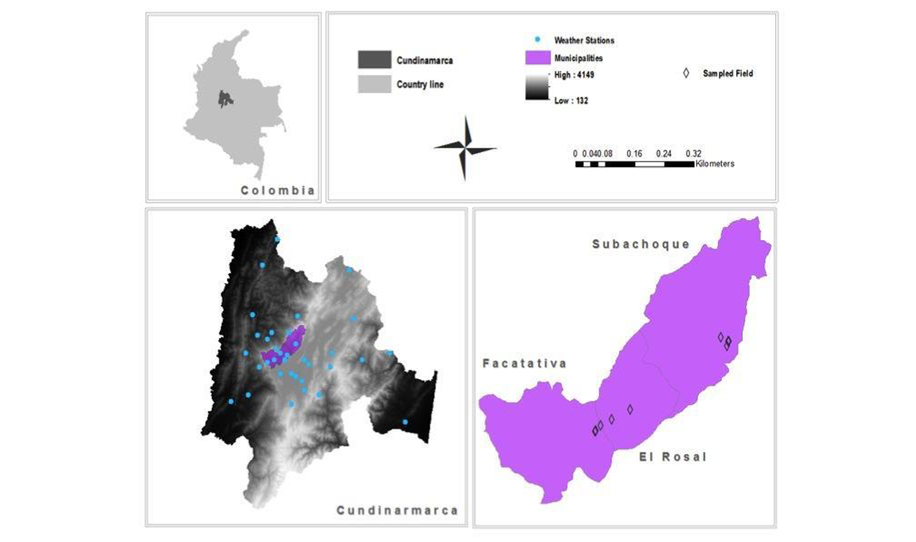
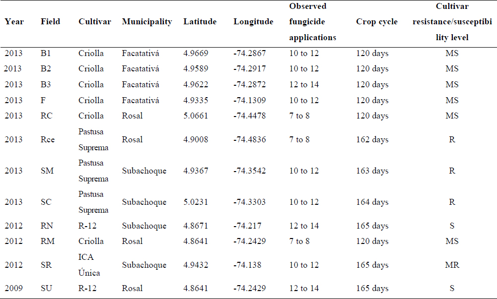
Late blight surveys and samplings were carried out at several locations in three municipalities of the department of Cundinamarca, Colombia: El Rosal, Subachoque, and Facatativá (Table 1, Suppl. Fig. 1), with the consent of growers, field owners, and assigned agricultural extension agents of the Colombian Federation of Potato Producers (Federación Colombiana de Productores de Papa, fedepapa). The fields were chosen based on the following criteria: i) the potato varieties grown, and ii) days after emergence (i.e., days after germination). Due to commercial crop usage, fertilization and commercial fungicides and pesticides were applied according to the standard grower practice in each region. We sampled several potato cultivars (Solanum tuberosum and S. tuberosum group phureja), such as Diacol Capiro (R-12) (susceptible), Pastusa Suprema (resistant), Criolla Colombia (moderately susceptible), and ICA Única (moderately resistant) (Table 1). Tuber seeds were planted at different times of the year depending on the region. The same field could not be sampled during three yearsbecause of crop rotations.
Sporangia counts and climate variables during the epidemics
Samplings of late blight lesion sites started at crop emergence and then were performed weekly until harvest. We defined two transects within the plot; 6 to 9 samples were collected in each location on each sampling day (Table 1). A sample consisted of ten leaflets; these were placed into a 50 ml sterile tube with sterile water. Sporangia counts were performed in duplicate using a hemacytometer. These data were used to evaluate the dispersal capacity of the pathogen over time.
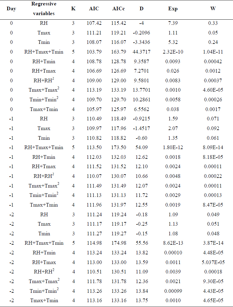
To assess the relationship between meteorological variables and pathogen dispersion (e.g., the amount of sporangia), we used several linear models in R v. 3.0 (R Core Team, 2018), as well as Granger correlations based on time shifts in certain cases (Granger, 1969) to fit climatic data (see below) and sporangia counts. The influence of climate variables on sporangia production was determined by evaluating ten linear models using the Akaike Information Criterion (AIC) (Suppl. Table 1). Models included relationships between sporangia counts and each variable or combinations of variables on the day of collection or one or two days prior to the collection day.
Climate data assessment and systematization
The spatialization of weather stations—which belong to the national catalogue of the Corporación Autónoma Regional (car) and ideam—was carried out using ArcGIS (Esri, 2009) to select the stations closest to the collection fields. Daily climate data from 66 stations were provided by ideam (Agreement 018/2011), and data from another 12 stations were provided by car (Suppl. Fig. 1). The data were organized in a relational database using the MySQL database manager. The database consisted of five tables; four tables summarize four climate variables: i) Rainfall, ii) Relative humidity, iii) Maximum temperature, and iv) Minimum temperature, for every day of the selected years. A relational table contains information associated with the stations, such as latitude, longitude, and elevation. This new table was linked to the previous tables, so that the geographical location and climate variables of any given station could be easily retrieved. Data interpolation was performed to determine the climatic behavior for each study area (see below). These data were included in a table linking climatic data and spatial information.
Climate data: Analysis and processing
A multiannual climate analysis was performed using data from car and ideam databases. Monthly data were selected if they met the following criteria: i) sampling location is more than 500 m from a water body, and ii) data records exist for over 30 years. As a result, 43 stations were selected for rainfall data, and 18 of the selected stations included variables related to humidity and average temperature. To determine long-term patterns in climate variables, we performed a multiannual analysis of data over a 30-year period in the selected area. To complete this, missing data were interpolated using average values of the same variables for other years. A monthly multiannual table was calculated for every month of the year.
For this analysis, we took into consideration only stations for which variables such as rainfall, relative humidity, and average temperature were available. To illustrate the overall behavior of the features, we simultaneously plotted average temperature, rainfall, and relative humidity in a chart where one axis represents the scale of temperature and rainfall, and the other axis represents relative humidity. This presentation was useful to study the relationship between these variables to describe the climatic conditions of each site. It was possible to create a map using the geo-referenced data provided by car and ideam databases to select the stations that better cover the study area. This map was processed using ArcGIS, and the “El Niño-La Niña Southern Oscillation” years were selected according to the severity classification provided by the ideam’s Atlas Climatológico (Climate Atlas) (ideam, 2006), which helps to determine the beginning and the end of the anomalous years.
Nonetheless, the GeoSimCast model requires more information to trace the behavior of the studied weather variables for the sampled fields. To generate these data, we applied an interpolation method using the anusplin software (Hutchinson, 2004). This software is based on spline models and allows the allocation of data over a geographical surface; it performs well and has been used in previous studies (Giraldo et al., 2010). Using the SplineA console, we assessed each station as a data point; the regressor variables considered are the meteorological features to be evaluated (e.g., rainfall), geographical coordinates (e.g., latitude and longitude), and the altitude in meters above sea level. The model extracts, by location, the climate conditions during the three study years according to the sampling time. The estimated surface represented data in a grid of 85 rows and 74 columns. The output files were in ascii format, where the header described the surface area and the number of points in the grid. These files were converted to raster format using model builder in ArcGIS v 10.1. After that, the daily climate data of each field were extracted from the weather surface using the ArcPy Python module by ArcGIS.
GeoSimCast
GeoSimCast is a program based on the Java programming language (Giraldo et al., 2010). This program uses an algorithm to obtain SimCast variables and run a SimCast forecast model over weather surface data. The weather surface is coded with a matrix of numbers representing colors (number of fungicide applications during each year) and coordinates. In gis, these weather surfaces or matrices can be visualized as agroclimatic risk maps.
SimCast is a forecast model used in potato late blight disease (Fry et al., 1983) that can help predict the optimal timing of fungicide application to potato crops. For daily data, it uses three weather variables: the number of hours above a humidity threshold, temperature during the same period, and rainfall. The first two variables rate disease severity as blight units (BUs), while rainfall quantity, represented as fungicide units (FUs), is related to how much active ingredient is washed from the leaves. After an accumulated threshold of BUs or FUs, the model recommends the optimal timing of sprays. ArcGIS processed the resulting maps with the Map Algebra toolset to compare differences in area between cultivars and thresholds in the models.
Results
Climatic conditions and disease
Sporangia curves as a measure of dispersal potential
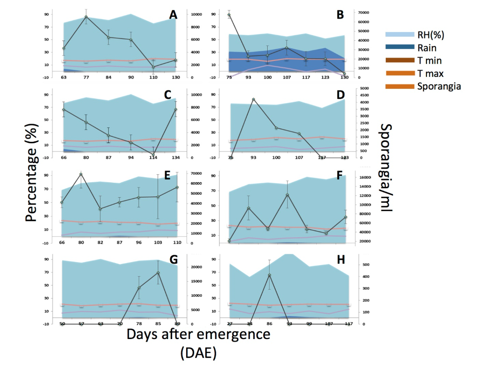
Differences in the sporangia curves were observed between fields in the initial amount of sporangia (IAS) and the curve trend (Fig. 1). The highest value for IAS was 68,125 sporangia/ml for R-12, a susceptible cultivar sampled in 2009 (Fig. 1B), followed by B1 with 47,638 sporangia/ml, a moderately susceptible cultivar sampled in 2013 (Fig. 1E); the lowest value was 0 sporangia/ml for a resistant cultivar sampled in 2013 (Fig. 1H).
Figure 1.
Sporangia curves of late blight pathogen based on samplings in different locations and cultivars during 2009, 2012, and 2013. Climate conditions are depicted. Left axis corresponds to % of relative humidity and the right axis to the number of sporangia/ml. A) A field in the Subachoque region sampled in 2012 with the cultivar R-12. B) A field in the El Rosal region sampled in 2009 with the cultivar R-12. C & D) Fields sampled in 2012 with varieties ICA Única in the municipality of Subachoque and Criolla in the El Rosal municipality. E & F) Criolla cultivar fields sampled in 2013 in the region of Facatativá. G) Criolla fields sampled in 2013 in the region of El Rosal. H) Field of the Pastusa Suprema cultivar sampled in 2013 in the region of Subachoque.
Source: Elaboration by the authors.
Superimposing sporangial curves on the climographs allowed us to extract some trends (Fig. 1). In El Rosal, the cultivar R-12 (susceptible) sampled in 2009, and in Facatativá, F field, the Criolla cultivar (moderately susceptible) sampled in 2013 had the highest values of sporangia/ml throughout the crop cycle (Figs. 1B and 1E, respectively). The high amount of sporangia in 2009 was correlated with the lowest values of minimum temperature. Low rainfall values were consistent for several fields in 2013 (Figs. 1E, 1F, 1G, and 1H), although the number of sporangia was consistently high in the Criolla cultivar (Figs. 1E, 1F, and 1G). The lowest amounts of sporangia were observed in the resistant cultivar (Pastusa Suprema) sampled in 2013 (Fig. 1H).
Weather conditions and their effects on sporangia production
This study was conducted in 2009, 2012, and 2013, and according to an official report of ideam, 2012 and 2013 were considered as regular years, while 2009 was an anomalous year (ideam, 2012).
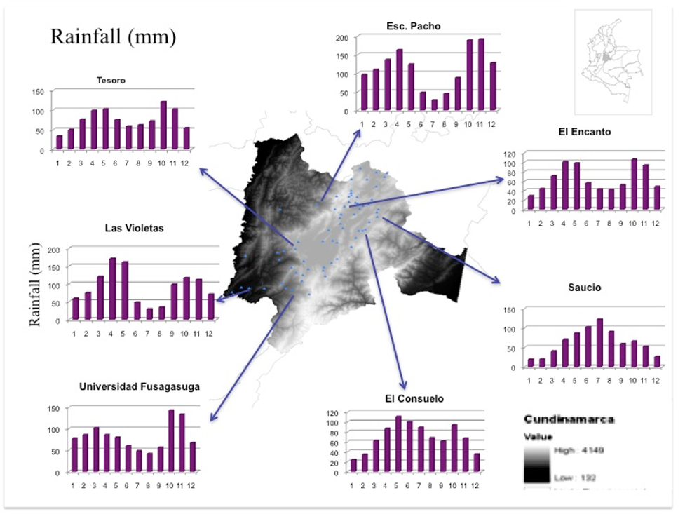
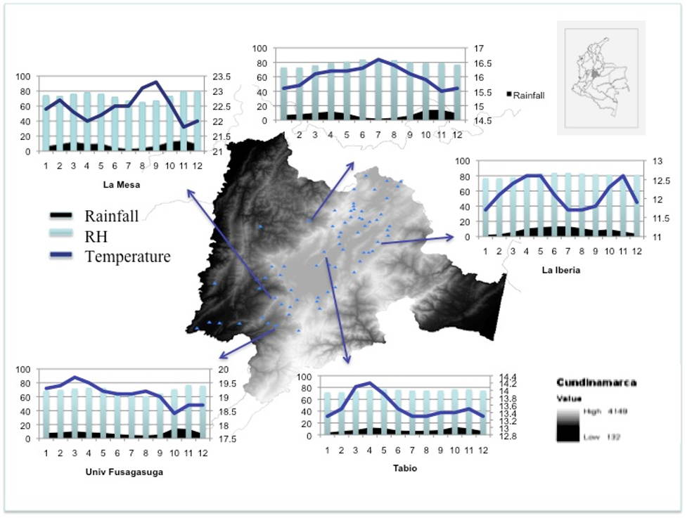
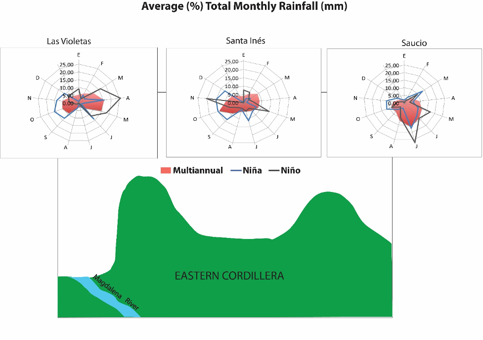
The eastern mountain range traverse the department of Cundinamarca, forming two clearly distinguishable rainfall regimes (Suppl. Fig. 2). We found rainfall to be monomodal on the eastern slope of the Cordillera, as revealed by the Saucio and El Consuelo stations, whereas the central plain and the western slope were characterized with a bimodal regime. Bimodal regimes had the first peak of rainfall between April and May, whereas in the second semester the peak was between November and December; the months with less rainfall were February, March, June, and July (Suppl. Fig. 2). The relative humidity was very similar throughout the department with an average between 60% and 80%, while temperature was very variable throughout Cundinamarca (Suppl. Fig. 3).
The relationship between different climate variables was determined based on the multiannual analysis. The climographs for weather stations depicted long-term climate conditions and the interaction between variables. For example, as expected, relative humidity and rainfall, in most of the stations, were correlated. Temperature and rainfall showed a negative correlation except for the Tabio station where they increased in the same months (Suppl. Fig. 3).
We found differences in rainfall during normal and anomalous seasons; a comparison was performed between the multiannual calculation and values from the years when anomalies occurred. The following severe periods reported by ideam were used: from May 1997 to May 1998 for El Niño and from May 1988 to March 1989 for La Niña (ideam, 2006). The eastern slope showed a monomodal rainfall regime with a peak in July. During El Niño, there were several peaks in March, May, July, and October, followed by five months with less rainfall (Saucio station; Suppl. Fig. 4). During La Niña, there were three peaks through the year; the first peak occurred in March as with El Niño, a larger peak in July, and a moderate peak in October-November. In the central plain (Santa Inés station), due to El Niño, the rainy season was concentrated in two months, thus generating less rainfall in the next eight months, whereas during La Niña there were four months with more rain than the rest of the year (Suppl. Fig. 4). In the western slope (Las Violetas station), during El Niño, the rainy season was concentrated in the first semester of the year, leaving the other seven months with less rainfall; in contrast, La Niña concentrated rainfall in the second semester of the year with some exceptions that mitigated the dry season (Suppl. Fig. 4).
Significant correlation was found between weather variables and the behavior of pathogen sporulation capacity. The number of sporangia per field was influenced by relative humidity and maximum and minimum temperatures. A regression model considering these three variables as drivers of disease dispersion showed the lowest AIC in comparison to other models that considered different sets of weather variables (Suppl. Table 1). The maximum temperature had the greatest influence on data variation—low sporangia counts were associated with high temperatures. Data from 2009, 2012, and 2013 were fitted using this model. For 2009 and the cultivar R-12 (susceptible) sampled in 2012, the best model included data from the day before sampling (p-value = 0.02,** R = 0.9365); for 2012, with the potato cultivars Criolla and Única, the best model used data from the sampling day (p-value = 0.21, R = 0.8524; p-value=0.049,* R = 0.9667, p-value); additionally, for 2012 and the cultivar R-12, the best model included data from two days before sampling (p-value =0.1818, R=0.8748). Finally, for 2013, with the Criolla fields in the region of Facatativá, the best model showed a positive correlation with relative humidity and a negative correlation with maximum temperature (p-value= 0.012, R=0.93; p-value = 0.073, R= 0.82; and p-value=0.67, R=0.75).
GeoSimCast analysis
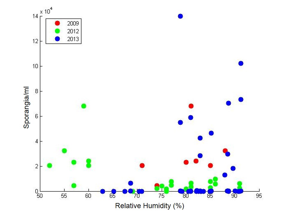
We evaluated the number of sporangia in different levels of relative humidity. We found that in 2012, the highest increase in the number of sporangia was found with approximately 60% relative humidity, and in 2009 and 2013, this increase was associated with approximately 85% relative humidity (Fig. 2). Notably, the number of sporangia outside a particular relative humidity range is consistently low for these three years, which suggests that the relationship between relative humidity and pathogen dissemination is non-linear. These data also show, as previously mentioned, that the production of sporangia does not depend only on relative humidity, but also on the interaction of variables and conditions prior to the day of collection. Based on these data, we set the simulation threshold for GeoSimCast greater than 60% relative humidity, and we also used a 90% relative humidity threshold, based on our multiannual climatic estimations and the suggestion that very high relative humidity is needed for the formation of sporangiophores (Fry, 2008).
Figure 2.
Different distributions of relative humidity in relation to pathogen dispersal capacity expressed as the number of sporangia/ml, over different years and in different cultivars. Different amounts of sporangia are correlated to different levels of relative humidity; in 2012, the highest number of sporangia were found with approximately 60% relative humidity, whereas in 2009 and 2013, the largest number of sporangia were found with approximately 80 to 90% relative humidity.
Source: Elaboration by the authors.
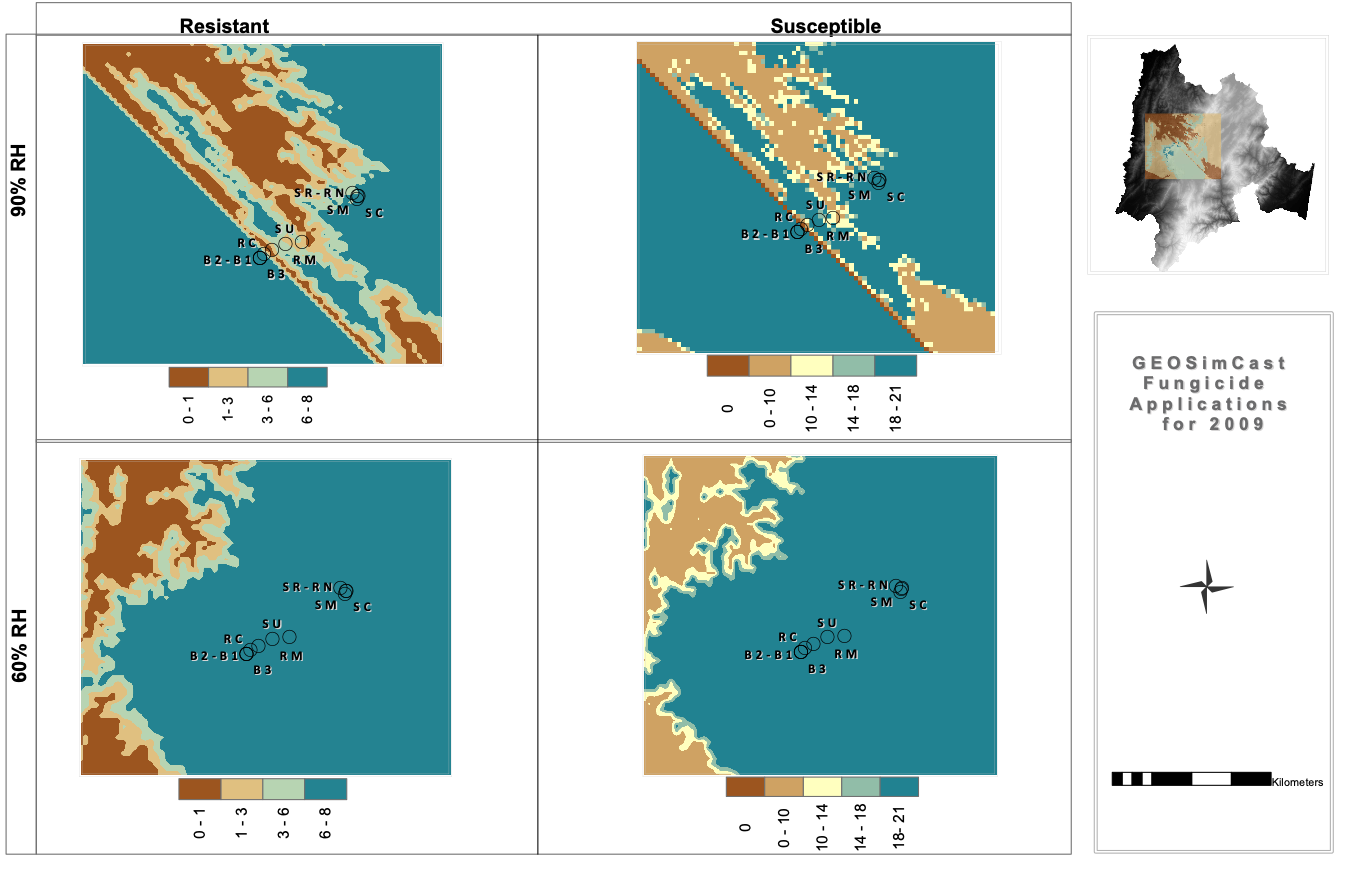
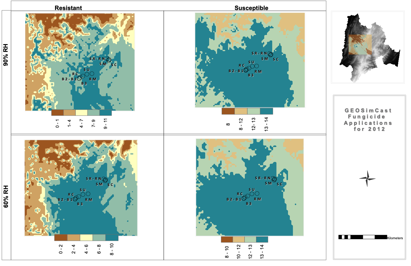
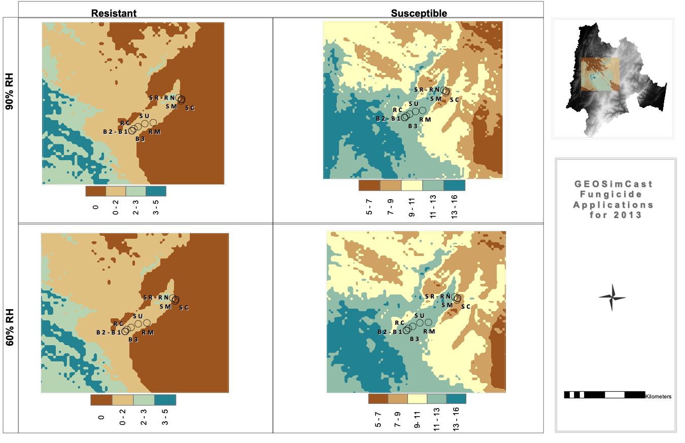
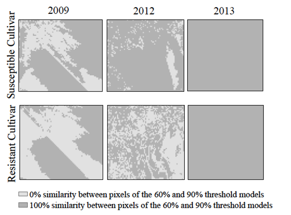
Agroclimatic risk maps showed disease severity in the area. Risk was represented by the number of fungicide applications during the crop cycle necessary to control the epidemic. In this analysis, two different types of cultivars were considered: one with high resistance and the other with high susceptibility. Similarly, two different thresholds of 60% and 90% relative humidity were used (Fig. 3 and Suppl. Fig. 5). We quantified the effects of different assumptions on the model by comparing areas of the two maps obtained under different thresholds (60% and 90% relative applications) (Fig. 3). In 2009, a large area of the map showed a constant number of fungicide applications; while susceptible cultivars showed a difference of 37% between the two models, resistant cultivars showed a preservation of 50% of the area for both models. For 2012, we found more variation between both thresholds: 12% similarity for the susceptible cultivar and 48.8% for the resistant cultivar. In contrast, in 2013, no difference between thresholds or cultivars was shown.
Figure 3.
Similarity between pixels for the 60 and 90% thresholds in GeoSimCast for the years 2009, 2012, and 2013 and different cultivars.
Source: Elaboration by the authors.
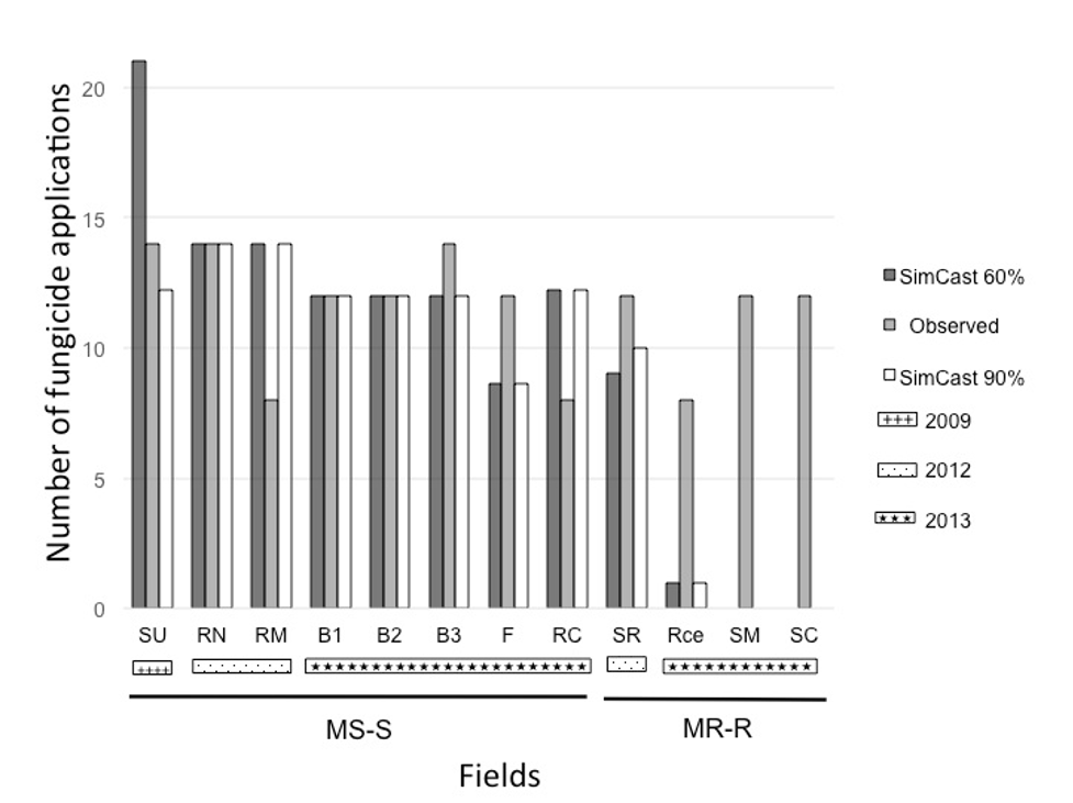
Not surprisingly, the cultivar grown determined the amount of fungicide applications estimated to control the epidemic in the models (Fig. 4). The 60 and 90% model runs suggested 0 to 1 application when using resistant cultivars in the sampled zone. This suggestion is consistently different from current data collected in the fields (7-14 applications). When considering the moderately susceptible and susceptible cultivars, the number of applications suggested by the two models was closer (even identical) to the observed number of applications (Fig. 4). In most fields, model runs at 60 and 90% relative humidity thresholds recommended the same number of applications, showing the influence of other climate variables on the number of sporangia produced by the pathogen.
Figure 4.
Comparison between the observed fungicide applications and applications predicted by GeoSimCast using two different relative humidity thresholds: 60% (red) and 90% (green). For susceptible cultivars (SU, RN, B1, B2, B3, and F), the observed applications are closer to those predicted by the model using a 90% relative humidity threshold. MR: moderately resistant; R: resistant; MS: moderately susceptible; S: susceptible.
Source: Elaboration by the authors.
As stated above, model runs using a 90% relative humidity threshold showed a similar number of applications indicated by the model and the number of applications performed by growers when using susceptible cultivars (Suppl. Fig. 5). However, the distribution pattern of the applications significantly changed, as two different zones were clearly differentiated for the Subachoque and El Rosal fields. In these fields, different fungicide regimes can be distinguished, and different municipalities show different propensities toward infection. For Subachoque, during the seeding time, the model suggested 6 to 8 applications for 60% and 90% relative humidity thresholds in resistant cultivars, but 18 to 21 applications for susceptible cultivars. Potato growers reported up to 12 to 14 applications. The predictions for El Rosal behaved differently from those for Subachoque—two nearby localities (Suppl. Fig. 1)—and while the growers applied fungicides 7 to 8 times in a season, the model suggested 0 to 10 applications with 90% relative humidity. Finally, for Facatativá, we estimated a requirement of 18 to 21 applications with 60% or 90% relative humidity in a susceptible cultivar; meanwhile, commercial growers applied fungicide 10-14 times during the season (Fig. 4 and Table 1).
Discussion
This is the first study in Colombia to follow weather variables in commercial and large potato crop fields with the purpose of exploring climate correlation with the dispersal potential of the late blight pathogen in an important seed-producing area. The limited availability and quality of data, compared to laboratory and greenhouse studies (Andrade-Piedra, Hijmans, Forbes et al., 2005;Andrade-Piedra, Hijmans, Juárez et al., 2005; Forbes et al., 2008; Grünwald et al., 2000; Harrison, 1992; Hijmans et al., 2000), makes this study challenging. Climate data collection is poorly centralized and automated in Colombia; thus, it is important to evaluate the epidemic models’ sensitivity to the characteristics of available data. The field has a myriad of different features that provide researchers with large sets of heterogeneous data, such as different cultivars, locations, and weather conditions. Thus, the generation of agroclimatic risk maps allows an adequate land planning and knowledge of long-term patterns, as well as estimating the state of weather variables in the seeding period and comparing these variables with calculated optimal weather states for the spread of the epidemic (Grünwald et al., 2003). Our final goal is to propose another tool for crop development that could help establish bridges between academics and potato growers.
The study zone was in the Cundinamarca plain in the eastern mountain range between two slopes. For this reason, most of the stations showed a bimodal precipitation behavior, having more rainfall in the first part of the year and a dry period of up to four months between rainy seasons, consistent with dry and wet season regimes in Colombia (ideam, 2006). Temperature did show variations across the year and the location and relative humidity values were higher in Subachoque and Facatativá than in El Rosal for the neutral years (2012 and 2013). This effect was accentuated during the El Niño phenomenon (data not shown). We propose that the use of global climatic features (seasonal recurrence) can help properly determine specific periods of sensitivity to infection, as well as changes in epidemic behavior in anomalous seasons.
Our hypothesis regarding the correlation between weather features and disease spread was tested using linear models to fit sporangia curves and variables such as temperature, rain, and relative humidity. It was possible to predict a relationship between relative humidity, maximum and minimum temperatures, and sporangia counts for each field. These weather variables largely explained the variability of data. In the sampled fields, variation ranged from 60 to 80% in relative humidity and from 15 to 22 ºC in maximum temperature. Interestingly, we found that the time lag of these variables had a very significant effect on the response. High humidity and low temperatures were correlated with low solar radiation, as previously reported (Mizubuti et al., 2000; Olanya et al., 2011). Solar radiation explains variation in sporangia counts, as it could increase the risk of disease outbreak (Mizubuti et al., 2000). However, this variable was not considered in our study but should be included in future studies. Also, nighttime is important for dispersion as low temperature data could be useful to determine which periods of the year present more risk of disease outbreak (Kanetis et al., 2010; Mizubuti et al., 2000; Olanya et al., 2011; Sunseri et al., 2002).
The non-linear relationship between sporangia and relative humidity is of great importance because sudden changes in relative humidity can be sufficient to trigger an epidemic under favorable weather conditions. We found that sporangial yield is favored within a certain range of relative humidity levels; this range may change, as observed in 2012, but the increased production of sporangia still occurs in a restricted range of relative humidity. Because specific relative humidity levels are necessary for pathogen dispersion, it is necessary to assess the effect of relative humidity on the microclimatic environment of P. infestans to better understand the conditions driving epidemics. As shown, the relationship may not be linear, such that the optimal conditions for pathogen proliferation may be more restricted, and management should therefore be intelligently targeted to avoid epidemics. A linear relationship of sporangial production with variables such as temperature was observed regarding some cultivars and time periods. Again, some of these relationships are better understood when analyzing climatic data one or two days before sampling, which could indicate that favorable conditions for pathogen dispersion and proliferation may arise, and the effect could be observed days after these conditions have been met.
Climatic variability throughout Cundinamarca and the sampled fields affected late blight incidence in the potato crop. The dispersal of sporangia depends on environmental conditions; zoospores lack specialized structures for survival and are thus susceptible to drying and solar radiation. However, sporangia are produced in large amounts on infected plant tissue and can be carried by wind to new locations (Sunseri et al., 2002). Favorable environmental conditions for dispersal are cool temperature (15 to 22 ºC) and high humidity (95 to 100%), which are observed in the sampling fields from seeding time until harvest. The sporangia production cycles of the pathogen showed a zigzag pattern with continuous increases and decreases in sporangia levels over time, which is consistent with aspects of its biology that determine reproduction waves over infection times (Olanya et al., 2011). The resistance of cultivars also affects the colonization of new plants: between cultivar Diacol Capiro R-12 (susceptible) and the other cultivars (resistant and moderately resistant), there was a difference of ~30,000 sporangia/ml when comparing the highest counts for each cultivar. Sporangia curves showed differences between fields that could be correlated with weather conditions and cultivar resistance.
The fungicide application model can be subject to several biases. One of the key points where bias can be introduced is the relative humidity threshold selection; we showed that different threshold selection can have different effects on the predictions of the model. Additionally, these variations largely depend on several climatic features; it is thus important to assess the proper selection of this parameter based on field data. Under homogeneous climatic conditions, the selection of the relative humidity threshold can have few effects, as observed in 2013 when the relative humidity had low variation and there were few differences in predictions under the two different thresholds and cultivars. In years where the variation was larger (e.g., 2012), more sporangia appeared in low levels of relative humidity; thus, the predictions of the two models had large variation, and a high threshold does not properly identify the climatic risk of infection.
Our GeoSimCast model showed that for 90% relative humidity and for resistant and susceptible cultivars in 2009, our fields were divided into two different zones. The Subachoque fields and a few fields in Facatativá were more susceptible to the disease than the El Rosal field. Potato growers applied more fungicide—up to 10-12 applications. This susceptibility is correlated with weather because it was an anomalous year (El Niño, a dryer year). During the first semester, there was a moderate rainfall peak, and after June, a dry season began; sporangia counts decreased until the growing season ended, making it unnecessary to apply more fungicide (ideam, 2006). However, growers do not consider climatic variability in the year, and they always assume optimal conditions (susceptibility) for pathogen development throughout the season and spray according to this assumption (observed number of fungicide applications). Differences in model predictions and over different assumptions such as relative humidity threshold show the need to better understand the effect of these variables to address epidemics more adequately in the field.
This is the first study to include commercial crop data to calibrate the GeoSimCast model. Experiments used to calibrate and validate SimCast models are often performed in small fields and with standard conditions in the lab (Andrade-Piedra, Hijmans, Forbes et al., 2005;Andrade-Piedra, Hijmans, Juárez et al., 2005; Forbes, 2008; Grünwald et al., 2002; Harrison, 1992; Hijmans et al., 2000). These studies do not account for the role of environmental variables in large fields or in fields with different cultivars throughout the area. Sampling across three years provided us with data on weather variability in planting times through the year. SimCast models of severity consider several microclimatic factors that are difficult to measure in the field. Estimating these factors based on global climate variables using GeoSimCast enabled us to calculate the severity of infection. Model predictions and cross-validation with field data expand the horizon of environment-dependent infection patterns (Grünwald et al., 2002).
P. infestans sporangia curves and climate variables can be used to predict late blight on potato tubers and to improve disease control. Hypothesis testing in the field greatly enables the formulation of useful recommendations for the optimal use of fungicides in each field. To obtain an accurate predictive model for Colombian crops, sporangia curves should be measured under a broad range of environmental conditions and locations and include solar radiation data in the analysis. Additionally, quantitative knowledge of the survival and spread of P. infestans sporangia is important to understand and manage late blight in commercial crops. The application of short and long-term climatic models can enable the prediction of epidemic dynamics that, integrated into agroclimatic epidemiology, would be very useful to applied agriculture. The conjunction of agroclimatic models (GeoSimCast) and climate models such as CCCma models (Canadian Centre for Climate Modelling and Analysis, 2013) could provide further insight on the distribution of late blight and the interaction between the plant and the oomycete to reveal the consequences of standard practices on late blight progression.